When developing a digital temperature measuring circuit, the purely mechanical aspects of the design have to be clarified first; however, these will not be considered here. This is followed by the electro-thermal ones. In this sense, the following questions need to be answered:
- What is the intended temperature range?
- Which level of measuring accuracy is required?
- Which type of temperature sensor is to be used?
- How large are the tolerances of the sensor's electrical characteristics?
- Which minimum bit rate should the A/D converter provide?
- How high does the sensor signal sampling rate need to be?
- How large are the values and tolerances of all other passive components within the application?
It is particularly important to determine the temperature range and measuring accuracy, as they determine the following steps. For example, the temperature range in this case should be from +25°C to +150°C, and the overall accuracy needs to be ±2°C. In these [and similar?] cases, two temperature sensors are available: A highly sensitive but non-linear thermistor and a resistance temperature device (RTD), e.g. a platinum sensor that is linear but less sensitive.
Choosing the right sensor: Not an easy decision
When choosing the right sensor, it is important to decide which one can be used to achieve the desired specifications. It is not enough to simply answer each of the questions listed above. Since the various parameters exhibit complex interactions with each other, i.e. they influence one another.
In general: The limiting factor of a system determines the accuracy. If this is unknown, it is of little use to reduce the tolerances of the remaining parameters to almost zero. If, for instance, precision thermistors are used with the aim of measuring the temperature with an accuracy greater than ±0.2°C and a simple 8-bit A/D converter is simultaneously used, it would impair the precision of the thermistors significantly. It would be the same the other way round, too: If a moderately precise sensor is used, the application of a 24-bit A/D converter makes only limited sense. If the smallest temperature differences are to be detected, an ADC with high differential linearity in conjunction with calibration algorithms is recommendable.
Another method to achieve the most accurate measurement possible is to use a class A platinum sensor (±0.15°C at 0°C) with a linear temperature characteristic. However, its temperature coefficient is lower than that of a thermistor, i.e. the measurement signal must be amplified. This requires additional hardware and brings further tolerances into play.
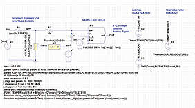
Obviously, this makes the selection of components a complex task, which usually demands numerous tests. And it costs time and money. It would be easier and faster if the sensor with its tolerances, the A/D converter accuracy, and the other hardware components could be selected, a "virtual prototype test system" set up, and a simulation carried out that immediately indicates the achievable accuracy. This is exactly what the PSpice-based simulation programs, which are mostly free of charge, do - even though they are analog simulation software. Since PSpice and its well-known "light" versions can simulate any process of the digital thermometer, as shown in Image 1 (in this case, a thermistor-based circuit, although an RTD-based circuit would look similar).
Components of the digital thermometer
Whether you choose an NTC (negative temperature coefficient) thermistor or a platinum RTD as your temperature sensor, SPICE models of these components are easy to find. In addition, the circuit contains a voltage divider consisting of a thermistor and a fixed resistor; a low-voltage source supplies the measuring current. The resulting voltage is digitized after amplification and filtering through the appropriate ADC. Ideal components are the new analog frontends from JRC (NJRC9103), which enable direct connection of the temperature sensor. This AFE supplies the digital data directly and also offers various calibration functions for offset compensation. A microprocessor utilizes this to calculate the temperature.
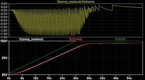
The direct transient circuit simulation (Image 2) shows the temperature profile of the application, the response of the sensor with a delay and slope, and the digitization of the signal. The time deviation of the readout temperature can be seen in the lower section. To make the digitization easier to recognize, a low A/D converter resolution of 10 bits and a long sampling time of 200ms were selected for the simulation.
The properties and tolerances of the sensor, in this example a 10k ±NTC thermistor of the NTCALUG series from Vishay, and the fixed resistor are easily simulated using Spice. The digitization of the signal and the conversion of the digitized raw measurement data into the temperature are carried out with the aid of analog behavioral modeling voltage sources. Interestingly, the number of bits (n) of the A/D converters is now a parameter of the simulation and can be varied between 8 and 24. The sample time (tone) of the sample/hold module is also a variable parameter. When using Sigma Delta ADCs, the external sample/hold can be omitted, especially since the temperature change typically occurs in the range of 100ms anyway.
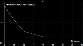
In this example, the sampling time of 10ms is the first parameter to be set. The ideal A/D converter resolution can then be determined by entering values between 8 and 24 bits. When calculating an error function as the effective value of the difference between the readout temperature and the thermistor temperature, the error does not decrease further at resolutions of n>16, as shown in Image 3.
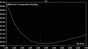
Alternatively, the series resistor R1 can also be optimized to achieve a minimum error value. Image 4 illustrates that the error function for an Rs series resistor reaches its minimum at 4.7kΩ. The ERR (error) function was defined in the SPICE directives for the simulation (see Image 1).
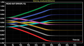
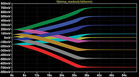
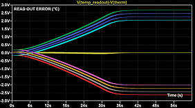
In the next step, the tolerances of the thermistor and the fixed resistor R1 are varied, and a worst-case analysis based on these tolerances is performed for each. Images 5 to 7 show three cases: Image 5 shows the results for an NTC with dR25/R25 = 1% and a B25/85 tolerance of 0.5%, combined with a 0.5% thin-film TNPW series flat chip resistor from Vishay. In this case, the measurement uncertainty increases from ±1.5°C at 100°C. The simulations apply to a worst-case scenario. Taking into account the R25 and B25/85 tolerances of the NTC and the tolerances of the fixed resistor R1, 2^3 = 8 cases are obtained; the white curve is the reference curve. The simulation in Image 5 shows that the tolerance values are evenly distributed; this means the relative tolerances of the resistors to each other have been chosen appropriately.
Image 6 shows that the temperature measurement uncertainty can be halved by halving all resistance tolerances (R25 = 0.5% and B25/85 = 0.25% for the thermistor and 0.25% for the fixed resistor). However, this is a somewhat ambitious undertaking, as it is doubtful whether all resistor suppliers can guarantee a B25/85 value of ±0.25%.
A common value for the B25/85 coefficients is, e. g., 1.5%. If the same simulation is performed with the same values as in Image 5 but with a B tolerance of ±1.5%, the results shown in Image 7 are achieved. Due to the relatively large measurement inaccuracies at high temperatures, they indicate a suboptimal design. It can also be clearly seen that the results for the tolerance values of the worst-case analysis are also not distributed ideally.
This shows that: A relatively simple simulation circuit can be used to visualize the overall accuracy of the temperature measuring circuit in line with its component dimensioning. This is an ideal starting point for additional experiments in order to reduce time and costs.
The simulation files used here can be requested from <link edesign.ntc@vishay.com - mail "open internal link">edesign.ntc@vishay.com</link>.
